One Dimensional Motion

Below is the one dimensional kinematic equation that we learn in physics class.
Given the initial position x1, initial speed v1 and acceleration a, the x2 position at time t can be calculated using the following formula.
\[v_{2} = v_{1} + a \cdot \Delta {t}\] \[x_{2} = x_{1} + v_{1} \cdot \Delta {t} + \frac{1}{2} \cdot a \cdot (\Delta t)^2\]Now we can use Python to calculate and visually see the result. These are the starting values:
- t = 100 seconds
- x1 = 4000 meters
- v1 = 500 m/s
- a = -10 m/s^2
1
2
3
4
5
6
7
8
9
10
11
12
13
14
15
16
17
18
19
20
21
22
23
24
25
26
27
28
29
30
31
32
33
34
35
36
37
38
39
40
import matplotlib.pyplot as plt
#parameters
x1 = 4000
v1 = 500
a = -10
t = 0
dt = 1
#generate a 100 second list to be used as time
tlist = [x for x in range(0, 100, dt)]
#list for velocity at time tlist[i]
vlist = []
#list for x positions at time tlist[i]
xlist = []
for t in tlist:
v2 = v1 + a * t # append to the list for velocity data
vlist.append(v2)
x2 = x1 + v1*t + .5*a*t**2
xlist.append(x2) # append to the list for y-position data
#comment out this line in trinket
fig = plt.figure(num=None, figsize=(12, 9), dpi=80, facecolor='w', edgecolor='k')
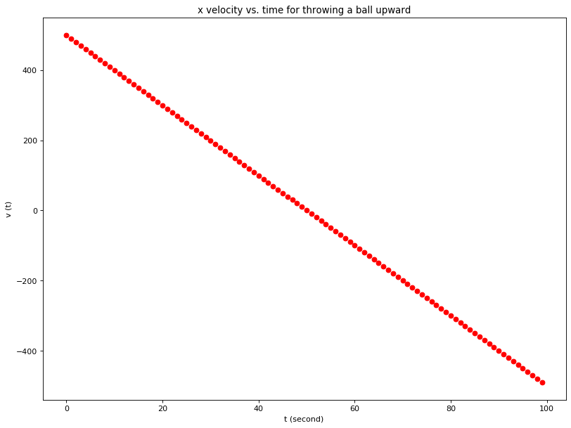
plt.title('x velocity vs. time for throwing a ball upward')
plt.xlabel('t (second)')
plt.ylabel('v (t)')
plt.plot(tlist,vlist,'ro')
plt.show()
#comment out this line in trinket
fig = plt.figure(num=None, figsize=(12, 9), dpi=80, facecolor='w', edgecolor='k')
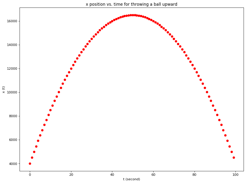
plt.title('x position vs. time for throwing a ball upward')
plt.xlabel('t (second)')
plt.ylabel('x (t)')
plt.plot(tlist,xlist,'ro')
plt.show()